Start
In this example, you generate labels on a mock dataset of transactions. For each customer, you want to label whether the total purchase amount over the next hour of transactions will exceed $300. Additionally, you want to make your predictions one hour in advance.
[1]:
import composeml as cp
Load Data
With the package installed, load the data. To get an idea on how the transactions looks, preview the data frame.
[2]:
df = cp.demos.load_transactions()

df[df.columns[:7]].head()
[2]:
| transaction_id | session_id | transaction_time | product_id | amount | customer_id | device | |
|---|---|---|---|---|---|---|---|
| 0 | 298 | 1 | 2014-01-01 00:00:00 | 5 | 127.64 | 2 | desktop |
| 1 | 10 | 1 | 2014-01-01 00:09:45 | 5 | 57.39 | 2 | desktop |
| 2 | 495 | 1 | 2014-01-01 00:14:05 | 5 | 69.45 | 2 | desktop |
| 3 | 460 | 10 | 2014-01-01 02:33:50 | 5 | 123.19 | 2 | tablet |
| 4 | 302 | 10 | 2014-01-01 02:37:05 | 5 | 64.47 | 2 | tablet |
Create Labeling Function
Define the labeling function that returns the total purchase amount given a hour of transactions.
[3]:
def total_spent(df):
    total = df['amount'].sum()
    return total
Construct Label Maker
With the labeling function, create the LabelMaker for this prediction problem. To process one hour of transactions for each customer, set the target_dataframe_index to the customer ID and the window_size to one hour.
[4]:
label_maker = cp.LabelMaker(
    target_dataframe_index="customer_id",
    time_index="transaction_time",
    labeling_function=total_spent,
    window_size="1h",
)
Generate Labels
Automatically search and extract the labels using LabelMaker.search().
[5]:
labels = label_maker.search(
    df.sort_values('transaction_time'),
    num_examples_per_instance=-1,
    gap=1,
    verbose=True,
)

labels.head()
Elapsed: 00:00 | Remaining: 00:00 | Progress: 100%|██████████| customer_id: 5/5
[5]:
| customer_id | time | total_spent | |
|---|---|---|---|
| 0 | 1 | 2014-01-01 00:45:30 | 914.73 |
| 1 | 1 | 2014-01-01 00:46:35 | 806.62 |
| 2 | 1 | 2014-01-01 00:47:40 | 694.09 |
| 3 | 1 | 2014-01-01 00:52:00 | 687.80 |
| 4 | 1 | 2014-01-01 00:53:05 | 656.43 |
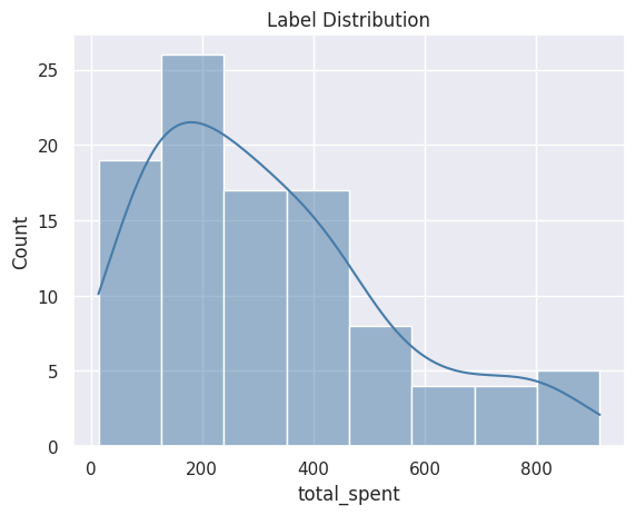
[6]:
%matplotlib inline
plot = labels.plot.dist()
Transform Labels
With the generated LabelTimes, apply specific transforms for our prediction problem.
Apply Threshold on Labels
To make the labels binary, LabelTimes.threshold() is applied for amounts exceeding $300.
[7]:
labels = labels.threshold(300)

labels.head()
[7]:
| customer_id | time | total_spent | |
|---|---|---|---|
| 0 | 1 | 2014-01-01 00:45:30 | True |
| 1 | 1 | 2014-01-01 00:46:35 | True |
| 2 | 1 | 2014-01-01 00:47:40 | True |
| 3 | 1 | 2014-01-01 00:52:00 | True |
| 4 | 1 | 2014-01-01 00:53:05 | True |
Lead Label Times
The label times are shifted one hour earlier for predicting in advance by using LabelTimes.apply_lead().
[8]:
labels = labels.apply_lead('1h')

labels.head()
[8]:
| customer_id | time | total_spent | |
|---|---|---|---|
| 0 | 1 | 2013-12-31 23:45:30 | True |
| 1 | 1 | 2013-12-31 23:46:35 | True |
| 2 | 1 | 2013-12-31 23:47:40 | True |
| 3 | 1 | 2013-12-31 23:52:00 | True |
| 4 | 1 | 2013-12-31 23:53:05 | True |
Describe Labels
After transforming the labels, use LabelTimes.describe() to print out the distribution with the settings and transforms that were used to make these labels. This is useful as a reference for understanding how the labels are generated from raw data. Also, the label distribution is helpful for determining if we have imbalanced labels.
[9]:
labels.describe()
Label Distribution
------------------
False      56
True       44
Total:    100


Settings
--------
gap                                    1
maximum_data                        None
minimum_data                        None
num_examples_per_instance             -1
target_column                total_spent
target_dataframe_index       customer_id
target_type                     discrete
window_size                           1h


Transforms
----------
1. threshold
  - value:    300

2. apply_lead
  - value:    1h
Plot Labels
You can use plots to inspect the labels.
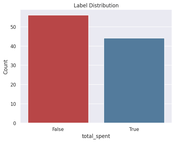
Distribution
This plot shows the label distribution.
[10]:
plot = labels.plot.distribution()
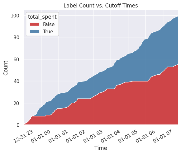
Count by Time
This plot shows the label distribution across cutoff times.
[11]:
plot = labels.plot.count_by_time()